
Sampling


Dataviz Team · Jean Russell
18 March 2021 · 9 min read
Sampling is the process of selecting a number of individuals to study from the entire population. In practice, it is often impractical if not infeasible to get hold of many entire populations due to many reasons such as the scale, time, and cost. A typical situation when it is impossible is when the population is theoretically infinite such as all the 5 year old cats in the world throughout time. However, even a finite population can take too long or be too expensive such as every household in Sheffield on a specific date. One of the most recent examples is the national census 2021 which is very complicated and time consuming. The answer is therefore to sample.
There are two types of sampling: random sampling and non-random sampling (you can also refer them as probability sampling and non-probability sampling). The former refers to sampling methods that draws samples from the population in accordance with the principle of randomisation where it does not carry any subjectivity. The latter are methods of extracting samples based on the researcher's opinions, experience, or relevant knowledge, therefore is subjective. Typical methods are convenience sampling, Voluntary sampling, snowball sampling, and selective sampling.
There are some key points to consider before building a model because we would like the characteristic of samples to be as close to the population as possible. We should always try our best to avoid sampling bias, reduce sampling error, and yield a true representative sample of the population.
In this material we will be looking at two sampling methods and ways to describe a sample. If you are also interested in how to sampling from a distribution using computational methods, visit the optional chapter Sampling - Computational Statistics.
Mean, Median, Mode, Range, Standard Deviation, Z-Score
None
In this section we will introduce you to two sampling methods - simple random sampling and selective sampling. If you would like to know other sampling methods, You might be interested in random sampling and non-random sampling.
The simple random sampling (and every other random sampling methods) ensures individuals in the population have equal probability of getting chosen. To ensure randomness, we usually assign individuals a unique number beforehand and use computers to generate random numbers, then choose individuals according to the generated number. However, very few sampling processes meet this criteria (equal probability). One reason is that in order to achieve you will need to have a listing for every single member of the population. There is therefore usually some systematic element to the sampling in a study.
Disadvantages: every individual is chosen at random but sometimes there is no way to ensure we have a representative sample for all subgroups.
The opposite to random sampling is selective sampling. Selective (or purposive, judgemental) sampling refers to when the researcher is familiar with his/her research field and has a good understanding of the overall survey, then a highly representative sample may be obtained by selecting objects/individuals entirely based on experiences. This sampling method is mostly used when the population is small and the internal differences are large, and when the overall boundary cannot be determined or because resources are limited. For example, a company wishes to investigate the tourism market in England, relevant departments select tourist spots such as London, Oxford, Cambridge, and York.
Disadvantages: Sample is greatly affected by the tendency of the researcher. If the subjective judgment is biased, it is easy to cause sampling bias. In addition, samples are not suitable to infer the overall population.
Here are two thought scenarioes we want you to take:
Hint: how many women are there normally on a physics degree?
It is particularly useful to think about who is excluded from a sampling technique. For instance, weekday park users might be very different from weekend park users.
Hint: How many students from Nigeria or Poland would be on Weibo?
Tool No.1. This tool provided by OnlineStatBook.com allows you to simulate sampling distributions. In the example shown below, the first graph is a customisable population distribution and in this case we have used mouse to created a very different distribution (pathological distribution). You can press the Animated button and it will draw a sample of size 5 by default. You can alter this using the third set of boxes down and select from 2, 5, 10, 16, 20 and 25.
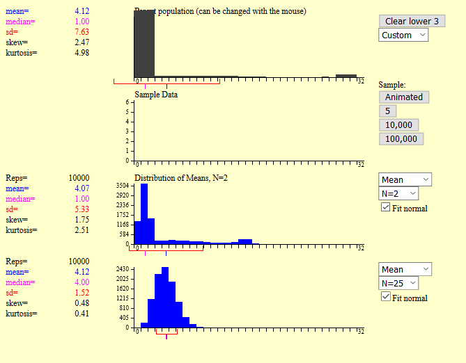
In the example shown above we drawn 10,000 samples of size 2 and size 25. You can see visually that when sample size is 2 the distribution cannot be identified or it is hard to say what distribution it has. When the sample size is 25 the sample mean distribution is slightly skewed, but you can tell it is following a Gaussian distribution. If the sample size is 100 then the mean will be following a Gaussian distribution and we'll see why (and the importance of Gaussian distribution) in Chapter 5 - The Central Limit Theorem. In this chapter you only need to know that sample means are approximately normally distributed if there is random sampling such that all units in the population are equally likely to be chosen. Why is this important? Imagine one of the few units at the right hand side of the graph have high probability of being selected, then this would make the sample mean be a lot higher than the population mean, which would make significant impact in most sampling techniques.
Tool No.2. The essycode website have a really useful tool that allows users to see probability mass/density functions and cumulative distribution functions for a range of probability distributions. You can also enter different parameters and distributions will be changed accordingly.
We also recommend you to use the Sample button at the top right corner of that website and try to generate samples in 10, 100, 1000, 10,000, and 100,000 to see the difference in the generated graphs. You will find that as the sample size increases, the sampling distribution generated at the bottom will approximate the theoretical distribution at the top. Samples are always discrete distributions but can approximate continuous distributions if the sample size is large enough.
Once we have samples from a distribution or a population, we should consider using some measures such as dispersion and central tendency to describe the characteristic of the samples. Samples from different distributions would likely be treated differently.
For samples from a binary variable, we can use the percentage (%) to get the ratio of two categories. For example, suppose the Dataviz.Shef has 1,290 visitors this month and we have a variable that tells us whether the visitor uses a mobile device to visit our website. We take five samples with a sample size of ten each and on average 3 people use mobile devices to visit the website. Then we can use 30% to describe this statistic instead of plain numbers.
For samples with multiple categories, consider using mode in addition to percentages. The mode will tell us what value/category has the highest proportion in the distribution. Note that the distribution can have more than one mode.
Similar to multinomial and binary variables, we should consider use percentages for ordinal data. However, median will be used instead of mode since categories are ordered in ordinal data and we are interested in the central tendency.
The choices for discrete data will be wider and more common. Some measures we can use are minimum, maximum, mean, median, and standard deviation. In addition, one might also consider interquartile range (IQR) and variance.
In addition to measures mentioned for discrete data, kurtosis and skewness are often used to describe the shape of the distribution. Kurtosis describes the tail of the distribution whereas skewness measures the asymmetry.
In this material we have seen different sampling methods and ways to describe samples. In the next part we will be looking at statistical models.