Introduction

This is the second blog post of the series Exploring packages in R. In this blog post we will explore some of the most popular packages in R for Static Visualisations. Same as in the previous blog post, I will be using the Hadfield Green Roof 5-year dataset and assume you already have some experience with R.

You can find all the source code in this Github repository. If you have any suggestions or want me to include any particular package feel free to send me an email!

In the next section we will explore ggplot2 - most popular package (according to download statistics) for visualising data, then followed by other alternative visualisation packages or packages that were built based on ggplot2.

ggplot2

The ggplot2 package is probably the most popular data visualisation package by downloads. There has been a lot of debate and comparison between the base plotting system and ggplot2 going on but I personally like ggplot2 more because:

• it allows much more customisation
• has unique ggplot layers which effectively decompose chart elements into functions and we can add layers on top of the existing chart
• and aesthetically pleasing

In general, if you mostly plot graphs for data exploring then the basic plotting will be sufficient. Whereas if your audiences are beyond yourself then ggplot2 works better. One thing to note is that ggplot2 doesn't support 3D plot at the moment. If you would like to know about the difference between them, check out this Comparing ggplot2 and R Base Graphics guide on FLOWINGDATA.

Most of the time we seek answers from the dataset we are approaching, and it is common we will have more questions pop up when examining charts for the dataset. I have prepared some questions to get started:

1. What is the difference in average temperature between consecutive winters (usually 20 Dec to 20 March, but the dataset is ended on 29 Feb 2016)
2. Correlation between each pair of variables
3. Density distribution of each variable
4. FAO-56 Penman-Monteith method
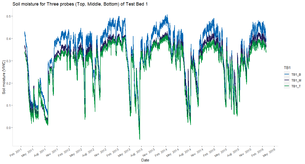
5. Is there a difference in VWC (soil moisture) between top, middle, bottom probe for testbed 1?

There are many functions available within the ggplot2 package, click here for the cheat sheet to see full options. There will be some pictures in this section, and I'll leave it to you to draw conclusions. It is also worth noting that you will find many specialised data visualisation packages depending on the ggplot2 package and building their functions around the ggplot2 object, therefore, a reasonable understanding of this package will add extra benefit when you explore other packages.

Bar chart

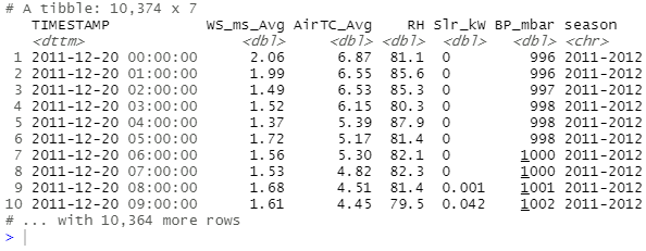
To get the date range out of the dataset, I'm using the between() function from the dplyr package. I'm also using | (the OR operator) for filtering multiple date ranges:

shefClimateNoNA %>%
  filter(
    between(TIMESTAMP, as_datetime("2011-12-20"), as_datetime("2012-03-20")) |
    between(TIMESTAMP, as_datetime("2012-12-20"), as_datetime("2013-03-20")) |
    between(TIMESTAMP, as_datetime("2013-12-20"), as_datetime("2014-03-20")) |
    between(TIMESTAMP, as_datetime("2014-12-20"), as_datetime("2015-03-20")) |
    between(TIMESTAMP, as_datetime("2015-12-20"), as_datetime("2016-02-29"))
  )

Since there isn't any variables that allows us to group dates in a convenient way, I'm going to create a new column called season for indicating which winter season each timestamp belongs to:

... %>% 
  mutate(
    season = if_else(
      month(TIMESTAMP) %in% c(11, 12),
      paste(year(TIMESTAMP), year(TIMESTAMP)+1, sep = "-"),
      paste(year(TIMESTAMP)-1, year(TIMESTAMP), sep = "-")
    )
  )  

The mutate() function adds the new variable/column season specified within the bracket to the dataset and each row value is conditioned on which month that timestamp belongs to. The paste() function allows us to join multiple strings using the separator specified at the end of the function.

That's great! Now we can group dates by seasons and calculate average temperature for each season!

... %>%
  group_by(season) %>%
  select(-TIMESTAMP) %>%
  summarise(across(everything(), ~mean(.x)))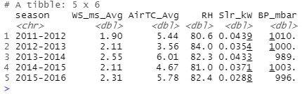 

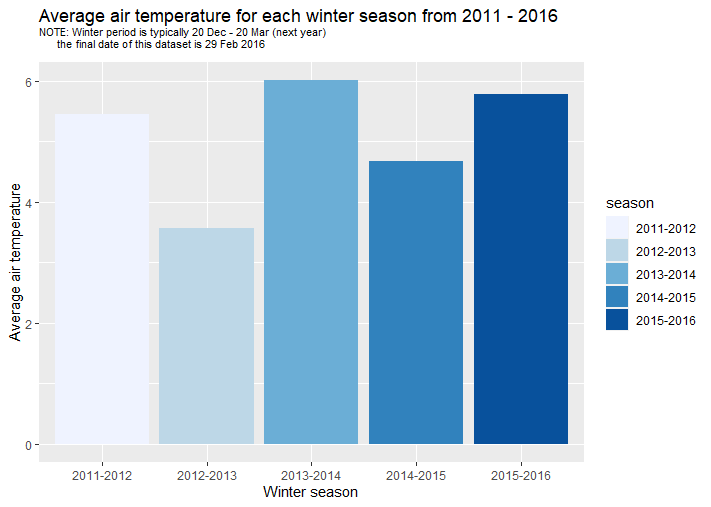
From the tibble shown above we can calculate the difference without an effort so I won't carry out the calculations here, but do remember that we don't have data beyond 29th Feb 2016. Instantly I can use ggplot2 to visualise the final outcome:

... %>%
  ggplot(data = ., aes(x = season, y = AirTC_Avg)) + 
  geom_col(aes(fill = season)) + 
  scale_fill_brewer(palette = "Blues") +
  labs(
    x = "Winter season", 
    y = "Average air temperature",
    title = 
      "Average air temperature for each winter season from 2011 - 2016",
    subtitle = 
      "NOTE: Winter period is typically 20 Dec - 20 Mar (next year)
      the final date of this dataset is 29 Feb 2016"
  ) +
  theme(
    plot.title = element_text(vjust = 1),
    plot.subtitle = element_text(size = 8, vjust = 4)
  )

Tile plane

The stats package has the cor() function for computing correlation:

corMatrix <- shefClimateNoNA %>% 
  select(-TIMESTAMP) %>% 
  cor() %>% 
  round(., 2)

corMatrix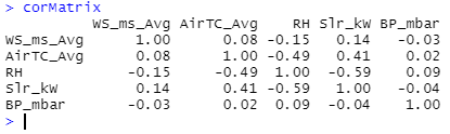

However, as you can see we are getting a matrix with row indexes being variable values and that's not what we want for ggplot() plus geom_tile() which requires three columns - two for the combinations of variables and the third column being the correlation value. So here are some transformations:

corVars <- rownames(corMatrix)

corMatrix %>% 
  as_tibble() %>% 
  # decrease the number of columns
  # add more rows
  pivot_longer(       
    cols=1:5, 
    names_to = "var1", 
    values_to = "value"
  ) %>% 
  mutate(var2 = rep(corVars, each = 5)) %>%
  relocate(var2, .after = var1)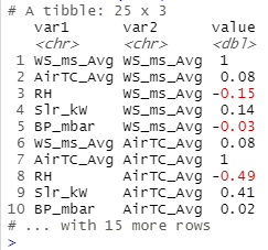

You can also install the reshape2 package commonly used to transform data into desired structures, but I will stick to functions within Tidyverse in this section to introduce you to as many functions as possible.

Now plot the graph:

... %>%
  ggplot(
    aes(x = var1, y = var2, fill = value)
  ) + 
  geom_tile(color="white", size=0.05) +
  scale_fill_gradient(low = "#fedf00", high = "#009640") + 
  geom_text(aes(label = round(value, 1)))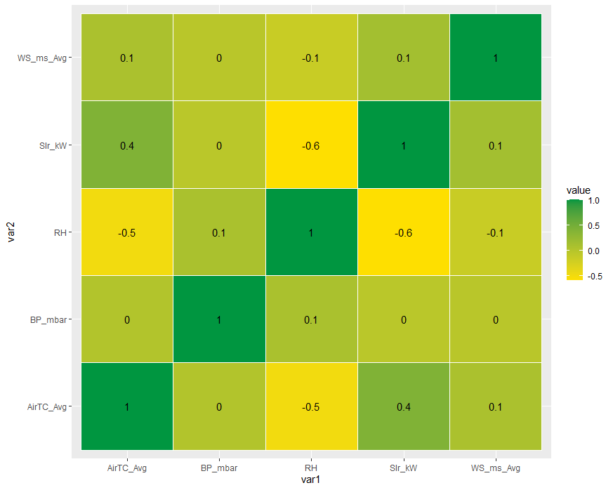

Density plot

To produce a density plot for each variable I simply repeat the function for each variable:

plot1 <- ggplot(data = shefClimateNoNA) + 
  geom_density(
    aes(x = WS_ms_Avg), fill = "#fedf00", color = "#fedf00", alpha = 0.8
  ) + 
  labs(x = "Average wind speed (m/s)", title = "Density plot for Average wind speed (m/s)")

# repeat for other variables
plot2 <- ...

plot3 <- ...

plot4 <- ...

plot5 <- ...

Then use the gridExtra package to arrange plots side by side:

library(gridExtra)

grid.arrange(plot1, plot2, plot3, plot4, plot5, ncol=2)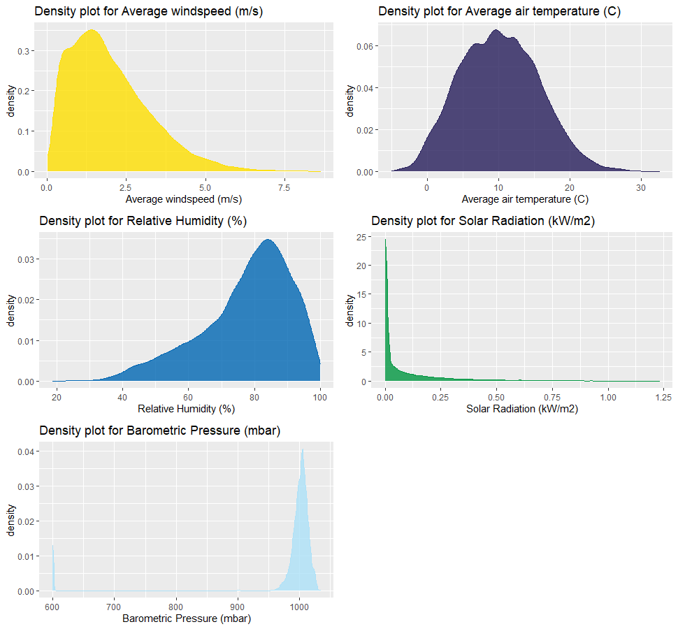

2D-bin

Move on to the FAO-56 Penman-Monteith method established to approximate the sum of water evaporation and transpiration from a surface area. I'm not an expert in Hydrology but thank to (Berretta, Poë and Stovin, 2014) and (Zotarelli, 2009) I was able to grasp some details in the formula and come up with the following (correct me if you discovered a mistake!):

Where

$X$ = $\frac{900}{24(T + 273)}(W(P - HP))$,
$W$ = Wind speed (m/s),
$T$ = Average air temperature (C), $Sr$ = Solar Radiation (MJ/m2/h),
$P$ = Pressure (kPa), and $H$ = Relative Humidity (expressed in fraction)

In the actual calculation I have made some adjustments to match the correct units:

• Convert solar radiation from kilowatt to joules we need 1W = 1J/s => 1kw = 1000J/s = 60,000J/min = 3,600,000J/hour = 3.6MJ/hour
• Convert pressure to kPa by dividing it by 1000
• Convert relative humidity to fraction

FAO56PM <- function(AirTC, solar_radiation, windSpeed, relativeHumidity, pressure, hourly = TRUE) {
  period <- if(hourly == TRUE) 24 else 1
  
  (0.408 * AirTC * solar_radiation + 
     0.066 * (900 / period / (AirTC + 273)) * 
     (windSpeed * (pressure - (relativeHumidity) * pressure))
  ) / 
    (AirTC + 0.066 * (1 + 0.34 * windSpeed))
}

shefClimateNoNA %>% 
  filter(between(TIMESTAMP, as_datetime("2011-03-01"), as_datetime("2012-03-01"))) %>%
  mutate(
    FAO56 = FAO56PM(AirTC_Avg, Slr_kW*3.6, WS_ms_Avg, RH/100, BP_mbar/1000)
  )

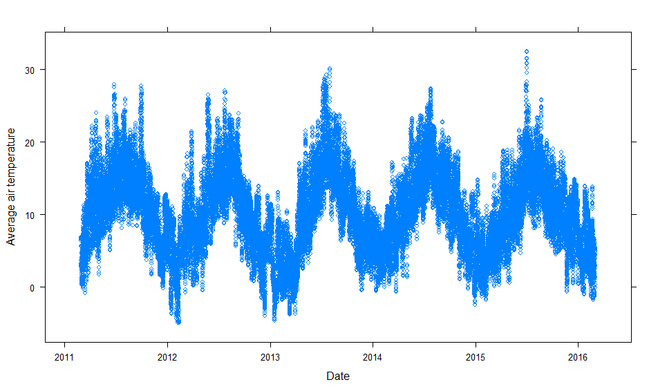
Now I'm going to use 2D bin to visualise the density of FAO56 values:

... %>%
  ggplot(aes(x = TIMESTAMP, y = FAO56)) +
  geom_bin2d()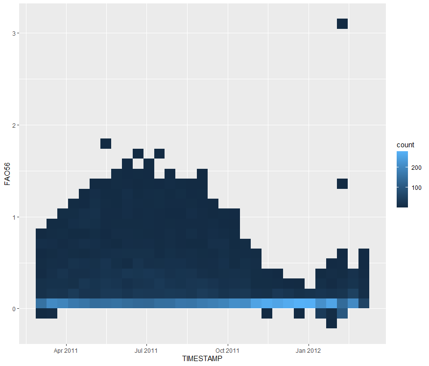

Time series

For this section I'm going to compare VWC (soil moisture) between top, middle, bottom probe for testbed 1, so let's read another dataset from the repository:

shefVWC <- read_csv(
  "https://figshare.shef.ac.uk/ndownloader/files/25647500",
  col_types = cols(
    col_datetime("%d-%b-%Y %H:%M:%S"),
    col_double(),
    col_double(),
    col_double(),
    col_double(),
    col_double(),
    col_double(),
    col_double(),
    col_double(),
    col_double(),
    col_double(),
    col_double(),
    col_double()
  )
)

My intention is to create a time series for each probe but also display them on the same graph and to achieve this I need to group values in a separate column (as the geom_line() function only accepts two variables). To achieve this, we can use the pivot_longer() function encountered before and create a new column which contains all values from columns TB1_T, TB1_M, and TB1_B. Then in the ggplot() function we specify the group parameter to be the new column and we're done! The last thing to do (as usual) will be styles, there are tones of customisation you can do to a chart and I encourage you to check out the ggplot2 cheat sheet.

shefVWC %>% 
  pivot_longer(cols = TB1_T:TB1_B, names_to = "TB1", values_to = "TB1value") %>%
  ggplot(aes(x = TIMESTAMP, y = TB1value, group = TB1, color = TB1)) +
  geom_line(size = 0.9) +
  scale_color_manual(values = c("#0066b3", "#251d5a", "#009640")) +
  labs(
    x = "Date", 
    y = "Soil moisture (VWC)",
    title = "Soil moisture for Three probes (Top, Middle, Bottom) of Test Bed 1"
  ) + 
  scale_x_datetime(
    date_breaks = "3 month", 
    date_labels = "%b  %Y", 
    limits = c(as_datetime("2011-03-01", tz="UTC"), NA)
  ) +
  theme(
    axis.text.x = element_text(angle = 30, hjust = 1),
    panel.grid.major = element_blank(),
    panel.grid.minor = element_blank(),
    panel.background = element_blank(),
    axis.line = element_line(color = "#dbdbdb")
  )

Other packages

In this section I'll briefly introduce some packages you can use as an alternative or in addition to ggplot2. Over the time there will be more great packages coming out so if you have any suggestions or want to include any particular package in this section feel free to send me an email.

ggpubr

The ggpubr package is based on the ggplot2 package and aims to empower researchers with no advanced R programming skills to create publication ready plots by providing a less opaque syntax. If you are new to R then it is worth a while to explore the package in more detail.

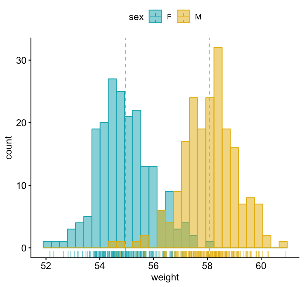Histogram with mean lines and marginal rug (source: ggpubr)

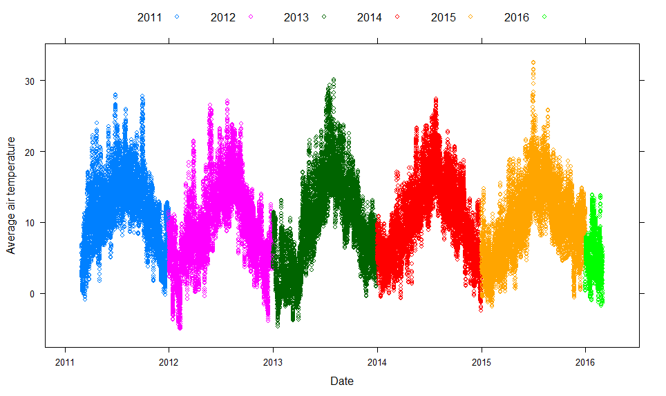
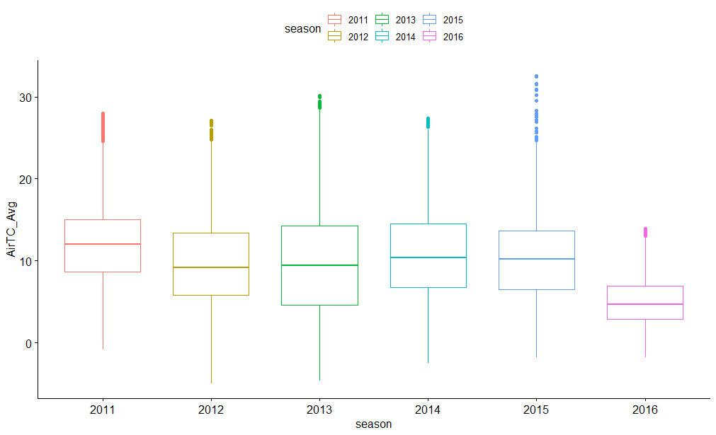Boxplots for each year's air temperatures

Lattice

The Lattice package was published a few years ahead of ggplot2 and although it might not be as popular as ggplot2 but it is however great for multiple plots on the same plane (via conditioning), simple 3D plots, or visualising multivariate data. However, styling is not intuitive and easy as you will find in ggplot2 since charts in Lattice cannot be stored as objects and there are no 'layers' you can add onto the chart once it is generated. The syntax in Lattice will look familiar if you have used Formula in R before, visit here to learn more about.

Some simple examples:

Simple relationship between variable x and y

Simple relationship between variable x and y with groups

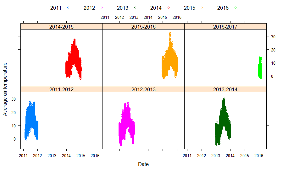Relationship between variable x and y for each level of z

rgl

rgl is a package specialised in 3D visualisations that also supports real-time interactive plots. It contains functions which allow users to convert graphics produced by rgl to Lattice or base. For more information on how to use rgl, see the following resources:

• rgl Overview
• A complete guide to 3D visualization device system in R
• rgl manual

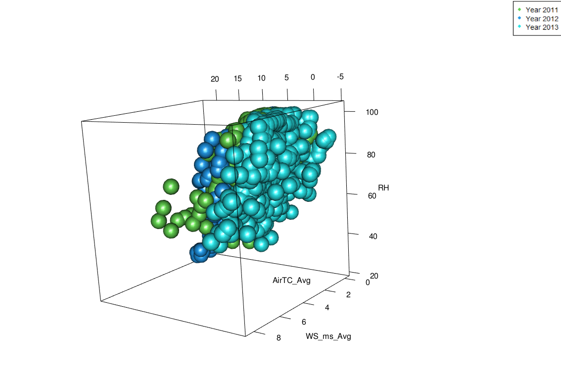3D plot (air temperature vs humidity vs wind speed) for Mar 2011, Mar 2012, and Mar 2013

esquisse

If you are new to R and like to use ggplot2 or have used it a lot then you might find esquisse useful when you don't want to spend time writing long codes or just want to explore the dataset real quick. This is an add-on package for RStudio and you can launch it via RStudio menu or execute esquisse::esquisser():

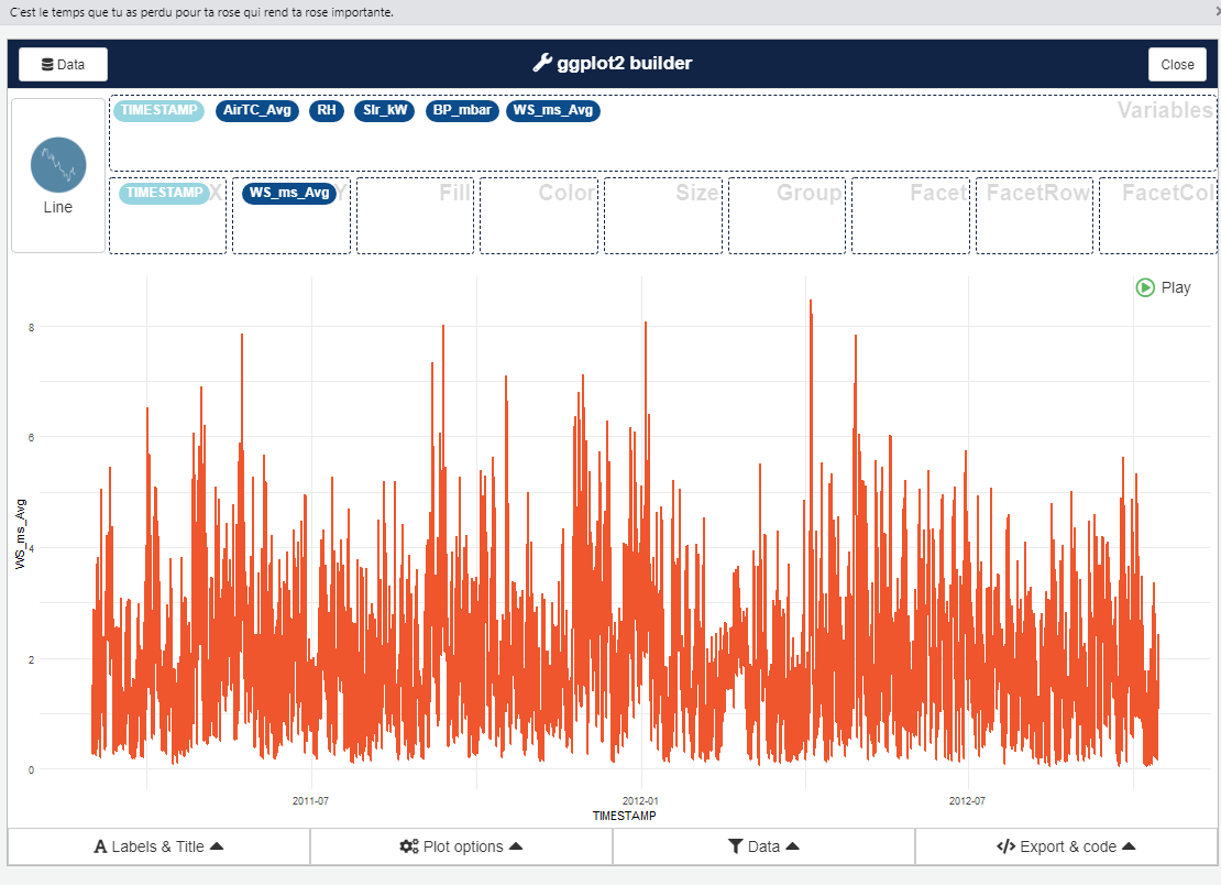
This add-on allows you to select data frames from the environment, choose most of the charts supported by ggplot2, specify parameters, filter variables, and many more via click, slide, drag and drop. Under the hood it uses ggplot2 and dplyr so features are limited and you will have to do the data transformation before feeding in data.

ggrepel

You will find ggrepel extremely useful if you regularly use text labels in ggplot2 and try to think of a better way to organise them without obstruction and overlap. I have used this package in the Moving from Excel to R blog post.

paletteer

If you want to access a range of colour palettes then the paletteer package should not be overlooked. If you are using ggplot2 then you can always use scale_color_paletteer_d() function on top of the existing charts.

What's next

The third part of this series will be on interactive plots and we'll be exploring packages such as Plotly, htmlwidget, and Shiny.

References

Berretta, C., Poë, S. and Stovin, V. (2014). Moisture content behaviour in extensive green roofs during dry periods: The influence of vegetation and substrate characteristics. Journal of Hydrology, 511, pp.374–386.

Zotarelli, L. (2009). AE459/AE459: Step by Step Calculation of the Penman-Monteith Evapotranspiration (FAO-56 Method). [online] Ufl.edu. Available at: https://edis.ifas.ufl.edu/ae459 [Accessed 14 Apr. 2019].